Custom Colormaps
Medical images typically store scalar intensity values, with each voxel storing a single value to report its brightness. A colormap transforms each voxel intensity to a color with four components: red, green, blue and alpha (opacity).
This page describes the NiiVue format for storing these transforms. NiiVue comes with many built-in colormaps. The colormap live demo allows you to explore these colormaps as well as define custom colormaps.
Basics
You can paste the code snippets below into the colormap live demo and press the custom button to see these colormaps in action. We define the red, green, blue, alpha (RGBA) values with 8 bits per component (0..255).
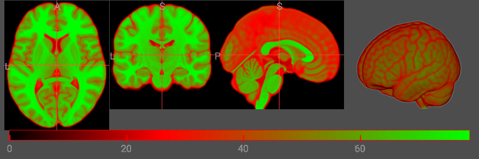
Consider a colormap that uses transpartent black (RGBA: 0,0,0,0) for the darkest intensity, opaque bright red (255,0,0,255) for intermediate values, and opaque bright green (0,255,0,255) for the brightest intensities. Therefore, this colormap has three nodes (black, red, green) and the resulting colormap could look like this:
let cmap = {
 R: [0, 255, 0],
 G: [0, 0, 255],
 B: [0, 0, 0],
 A: [0, 64, 64],
 I: [0, 85, 255],
};
Alpha
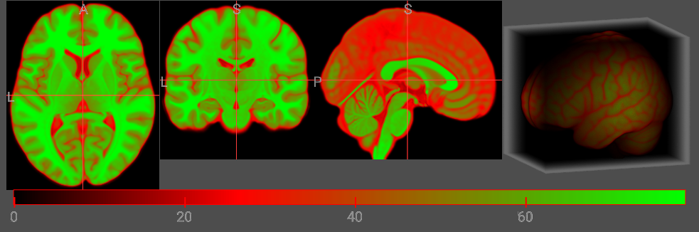
The Alpha component sets the opacity of the volume rendering. For most MR modalities, air has darker intensities than tissues, and we want to make the air transparent. Therefore, in the example above, the air is completely transparent (A: 0) while the brain is translucent (A: 64). In the example below, we make the air have a little opacity (A: 0). Notice the rendering shows the brain surrounded by haze.
let cmap = {
 R: [0, 255, 128],
 G: [0, 0, 128],
 B: [0, 0, 255],
 A: [6, 64, 64],
 I: [0, 85, 255],
};
Index
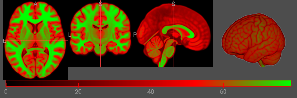
The least intuitive aspect of the colormap is the index component (I). This should be zero for the first node and 255 for the final node, and intermediate nodes placed between these two extremes. To visualize the influence of the node position, consider changing the position of the middle (red) node from 85 to 170. The colormap gradient still has the order black, red, green but the black-red portion is now larger and the red-green is now shorter.
let cmap = {
 R: [0, 255, 0],
 G: [0, 0, 255],
 B: [0, 0, 0],
 A: [0, 64, 64],
 I: [0, 170, 255],
};
Range (min..max)
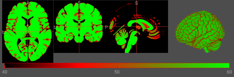
You can optionally specify the min and max range for the colormap. In the example below, this clamps the colorbar to the range 40..60. This is useful for CT images, where voxel intensity reflects calibrated Hounsfield Units. However, this is typically not useful for MR images, where most sequences generate relative intensities. Therefore, for MR the minimum and maximum can vary between images. When the image intensity range is not specified, NiiVue will set the default range of the colorbars to the robust range.
let cmap = {
 min: 40,
 max: 60,
 R: [0, 255, 0],
 G: [0, 0, 255],
 B: [0, 0, 0],
 A: [0, 64, 64],
 I: [0, 85, 255],
};
Shortcuts
All colormaps must specify the vectors Red (R), Green (G) and Blue (B). These three vectors must have the same number of elements as each other, and must have at least two elements and no more than 256 elements. If you do not specify the Indices (I), the nodes will be evenly between 0 and 255. If you do not specify the Alpha (A) the first node will have be transparent (A: 0) and all others will be translucent (A: 64). Therefore, the following is a valid colormap:
let cmap = {
 R: [0, 255, 0],
 G: [0, 0, 255],
 B: [0, 0, 0],
};
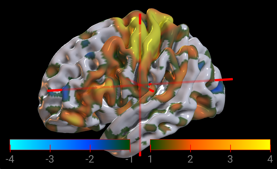
Negative Colormaps
Objects can specify both a positive and a negative color map. For example, this voxel-based image uses the warm colormap and the winter colormapNegative. Alternatively, this mesh uses the green2orange colormap and the green2cyan colormapNegative. This allows statistical maps to highlight correlated as well as anti-correlated contrasts.
Atlases and Labeled Images
The NiiVue colormaps described above are ideal for continuous images, but are not appropriate for indexed images such as atlases that have discrete tissues. The function setColormapLabel() allows you to override the previously described continuous colormap with a custom discrete colormap.
Consider an MRI scan that has been segmented with FSL FIRST. This can generate a volume where there are discrete tissues that we will want to map to specific colors and label with names. In this case, the segmented image may have the intensities 0 for Air, 1 for water, 2 for gray matter and 3 for white matter. This labeled live demo uses this colormap:
let cmap = {
 R: [0,   0, 120, 175],
 G: [0,  90,  60, 185],
 B: [0, 120,  60, 175],
 I: [0, 1, 2, 3],
 labels: ["air","CSF","gray","white"],
};
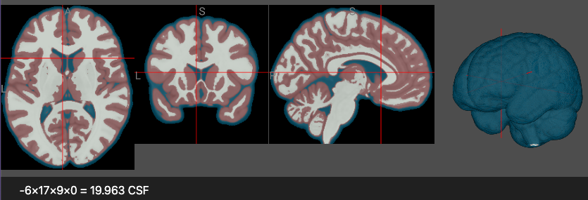
Note that each region can include a label, for example in the image the text reports that the crosshair points to a voxel with the CSF identity. The labels field is used to describe all regions.
Like continuous colormaps, the alpha (A) field is optional.
A major difference between indexed colormaps and continuous colormaps is that the indices (the I field) explicitly describes the intensity associated with a label. Labels can have more than 256 distinct regions, and the indices can be sparse. For example, consider an atlas image where the classes are air (0), CSF (1), Gray (2) and Whte (5), with the no voxels correspondong with intensity of 3 or 4. In this case, we could simply list the four discrete tissues defined:
let cmap = {
 R: [0,   0, 120, 175],
 G: [0,  90,  60, 185],
 B: [0, 120,  60, 175],
 I: [0, 1, 2, 5],
 labels: ["air","CSF","gray","white"],
};
The I field is optional: if it is not provided the labels are considered to be in the range of 0..n-1. Therefore, it is only required if the labels are sparse or do not begin from 0.
The labeled voxel live demo and labeled mesh live demo allow you to interactively change the colormaps.