Atlases
Atlases partition images into discrete regions, which may be defined by structural features, functional activity, arterial territories, or connectivity patterns. Some atlases are tailored to specific populations, such as pediatric or disease-specific cohorts. NiiVue supports a wide variety of atlas formats and types.
Voxel-based Atlases
NiiVue supports discrete voxel-based atlases, where each location in the brain volume is associated with a labeled region. In the embedded image below, you can see an example of this functionality. The opacity of the atlas can be adjusted using the slider, allowing you to view it in context with other data. Additionally, clicking on different locations will display the parcel name and its coordinates in the status area.
Mesh-based Atlases
Furthermore, NiiVue can load atlases onto meshes, providing similar functionality. This is illustrated in the below.
Probabilistic Voxel-based Atlases
While many atlases are discrete (assigning each voxel exclusively to a single region) others are probabilistic, allowing a voxel to represent a mixture of regions. Probabilistic atlases are particularly useful for capturing variability across individuals, as seen in population-based studies where regional boundaries may vary from person to person.
However, storing and visualizing probabilistic data can be computationally demanding. For example, version 3.1 of the Julich-Brain Atlas includes 207 regions and, when uncompressed in MNI space, requires 7575 MB of memory. To address this challenge, NiiVue uses the PAQD format (described here), which stores only the two most probable regions per voxel. This approach reduces the memory footprint dramatically—in this case, to just 8 MB—while retaining meaningful information for visualization.
The interactive graphic below demonstrates this format. When you click on a border area, the two most probable regions and their respective probabilities are shown in the status bar.
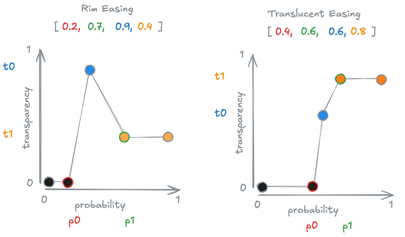
Additionally, a drop-down menu allows you to select different easing functions that convert regional probabilities into transparency values. For example, the Rim function renders border regions opaque and high-probability areas more translucent, whereas the Translucent function makes opacity increase with probability. These easing functions are governed by four parameters—p0, p1, t0, and t1—illustrated in the figure below. The horizontal axis represents probability, and the vertical axis represents transparency. Voxels with a probability below p0 are fully transparent. Voxels with a probability midway between p0 and p1 are assigned transparency t0, and those above p1 are assigned transparency t1. Transparency values between p0 and p1 are linearly interpolated.